Version 1.1. Fixed Figures 1 and 2, and accompanying text. If you can see a purple leaf in the diagram, your cache is showing you the old diagrams. Updated the text following Equation 2. Corrected typo in Equation 4. There are more revisions to come, as parts of this derivation are still very arm-wavy.

This post is meant to help create an intuitive feel for how the Lorentz transform works. I work through a number of simple steps, until in the end, an easy formulation of the Lorentz transform using the Clifford algebra is demonstrated.

I think I've got everything correct, however if you spot an error, or if something is not clear, or confusing, let me know in the comments!

The Lorentz transformation is used to convert measurements made by two observers into each other's frames of reference. Here are a couple of moving observers (figure 1); they're moving in x, y, z, in time, t.

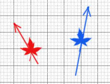 Figure 1

Each observer has an independent frame of reference. We'll denote the red observer's frame of reference the original frame, (x, y, z, t). The blue observer's frame will be (x', y', z', t').

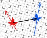Figure 2

At the given moment of time, we'll swing a common reference frame around such that the relative velocity between the two is on one axis, shown by the dark arrow in Figure 2. We can imagine as time goes on, the two observers will become more separated along this axis, commonly chosen to be z. The other two spatial dimensions are not changing. This is called the standard configuration. The Lorentz transformation relates how the two observers see each other. Since we've oriented things so that only the z axis is changing, we can use the Lorentz equation. The derivation of these equations are elegantly described in Einstein's famous 1905 paper (Reference 3), so I won't describe it here.

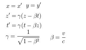Equation 1 

The Lorentz transformation describes how to go from one frame of reference to the other. If we graph the time on the vertical axis (it is traditional to do so), and the value we are measuring on the horizontal axis, as velocity increases, the prime frame of reference gets squashed along the diagonal (figure 3). When the relative velocity is zero, the two frames look the same; when the relative velocity is the speed of light, the prime frame collapses on to the diagonal.

Another way to think about this diagram is to realize that events on the vertical axis are events that occur at the same place in both frames but in different times. Events on the horizontal axis are events that occur at the same time in both frames but different places.

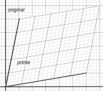Figure 3

If we generate a bunch of frames, and plot the same places and same times for the different relative velocities, we will discover that the shape of the transform is hyperbolic. To give an idea what that means, here is a hyperbolic surface (figure 4). Note that this isn't a solution of the equations, simply a visualization of what a hyperbolic surface could look like.

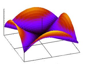Figure 4 

Here is the transform visualized another way (figure 5). If we imagine an event occuring at r = 0, and some t, for a given frame, that event will occur at the transformed location which can be found by tracing out the hyperbola until it intersects the frame (figure 6).

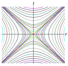Figure 5

Once again, the vertical axis represents time, the horizontal axis represents position. Position divided by time is of course velocity. The diagonals represent the speed of light, which never changes.

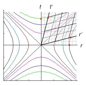 Figure 6

The red dots show events as they are transformed into the prime space.

At this point, it is traditional to generate a boost matrix to describe the transformation.

This matrix only gives a boost between two frames in relative motion. A full Lorentz matrix would also include rotations about the three axes. The matrix is already unwieldy, with rotations it becomes more so (see Reference 1).

For a different, and much easier approach, notice that the Lorentz transformation is actually a rotation in hyperbolic geometry! Figure 7 shows the hyperbolic functions. In the diagram, a is defined as the shaded area; it's analogous to regular trigonometric functions with the circle.

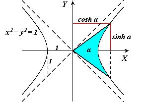 Figure 7

A hyperbolic rotation is therefore another way to think of the Lorentz transform.

 Figure 8

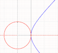Figure 8 demonstrates how the area of the hyberbolic function increases with a, as does the trigonometric function.

The following derivation follows Doran and Lasenby, reference 2. Referring back to Equation 1, we introduce a new identity:

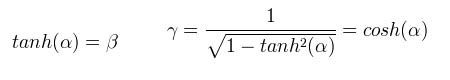 Equation 2

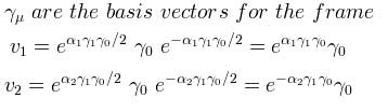
Next, we introduce some basis vectors, e, such that

In the prime frame, these basis vectors will be different; they will describe the transformed frame (recall Figure 3). The correspondence between the original and prime frames can then be expressed as

which we read as the original frame and prime frame are equivalent; the transformed and untransformed vectors are the same, and can be transformed in both directions - the transformation is covariant. Looking back at equation 1, we see that the x and y terms drop out and can be disregarded. Next, we derive the new frame in terms of the old:

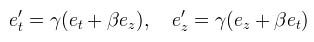
Substituting equation 2 through, we can re-express the relations as an exponential. The algebra we will use here is the Clifford algebra.

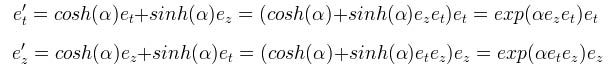
Now that it is in this form, it can be re-expressed as a rotor:

Equation 3

Note that last e is the natural e, not a basis vector. Finally, let's work an example (from reference 2). Suppose we observe two objects flying apart, what relative velocity do they see for each other? Recall the definition of a from equation 2, and the rotors of equation 3:

We derive the relative velocities

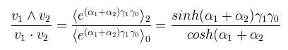Equation 4

We read equation 4 as: the relative velocity is the grade 2 components of the differential of the event vs. the proper time, divided by the grade 0 components of the time vs. the proper time as exponentials, which can be recast as hyperbolic functions, and evaluated as follows:

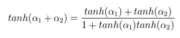
As a validation, replacing the hyperbolic tangents with u = c tanh(a) recovers the familiar equation from Reference 3:

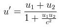
Which shows that addition of colinear velocities in space-time is the same as the addition of the hyperbolic angles - a generalized rotation in hyperbolic space!

References

1) Wikipedia article on the Lorentz Transform

2) Chris Doran and Anthony Lasenby, Geometric Algebra for Physicists, Cambridge University Press, 2003

3)Albert Einstein, On the Electrodynamics of Moving Bodies, Annalen der Physik, 17:891, 1905. The linked translation was prepared by John Walker.

The equations were created using an online LaTeX.

The diagrams were generated using Maxima.